Summary of Tutorial

This tutorial shows how to score raw item responses, compute CTT (classical test theory) statistics, compute fit statistics and plot expected scores curves.

The R script file for this tutorial can be downloaded through the link Tutorial4.R .

Data files

The data file is the same as for Tutorial 3, except that for multiple-choice items, raw responses are captured rather than scored responses. For example, if a student chose option 2 for Question 3, then 2 is recorded even though option 4 is the correct answer. The test paper and the data file can be downloaded through the following links:

To run an IRT analysis using TAM, the data need to be scored first.

R script file

Load R libraries

Before TAM functions can be called, the TAM library has to be loaded into the R workspace. Line 2 loads the TAM library.

Read data file

Line 5 sets the working directory and line 6 reads the data file "D1_resp.csv" into a variable called "raw_resp".
          setwd("C:/G_MWU/TAM/Tutorials/data")
          raw_resp <- read.csv("D1_resp.csv")

Score data file

Line 9 specifies the "keys" of the item responses.
          key <- c(1, 1, 4, 1, 1, 1, 1, 1, 1, 1, 3, 1, 1, 1, 1)
For example, for Question 3, "4" is the correct answer.

Line 10 scores an item response to "1" if the item response matches the key, otherwise scores it "0".
          scored <- sapply( seq(1,length(key)), FUN = function(ii){ 1*(raw_resp[,ii] == key[ii]) } )
The "sapply" function takes each row of "raw_resp" and matches it with the keys. 

Run IRT analysis (MML)

Line 13 runs an IRT analysis using MML estimation. The results of the IRT analysis are stored in variable "mod1".
           mod1 <- tam(scored)

Compute ability estimates

Line 16 computes the weighted likelihood ability estimates (WLE). The ability estimates and respondent test scores are stored in variable "Abil".
           Abil <- tam.wle(mod1)

CTT

After the IRT analysis is run, the ctt function can be called. Line 19 calls the tam.ctt function. The result of the function is stored in variable "ctt1".
           ctt1 <- tam.ctt(raw_resp, Abil$theta)
The "tam.ctt" function requires at least two arguments. The first argument is the item responses, whether scored or not scored. The second argument is either the WLE ability estimates or plausible values .

In the Console window, you can check the ctt results by typing "ctt1" followed by ENTER.
The output of ctt in the Console window is not always easy to read. You can write the output to a CSV file, as shown by line 20.
           write.csv(ctt1,"D1_ctt1.csv")

Below is an excerpt of the D1_ctt1.csv file.

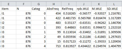
The columns of the D1_ctt1.csv file show item name, number of respondents, item category, response frequency, percentage, point-biserial correlation using WLE, the mean and standard deviation of WLE abilities for respondents in the response category.

As an exercise, you can run the ctt function for the scored data. For example,  ctt2 <- tam.ctt(scored, Abil$theta)

IRT person separation reliability

IRT person separation reliability is stored in the WLE.rel variable (see pdf document on tam.wle). To retrieve it, type
           Abil$WLE.rel
For this data set, the person separation reliability is 0.78.

Iitem fit statistics

Item fit statistics can be obtained after IRT analysis is run (see pdf document on tam.fit). The residual-based item fit statistics are produced. Line 23 of the R script file computes the item fit statistics.
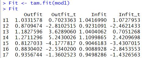
           Fit <- tam.fit(mod1)
The following is an excerpt of the fit statistics.

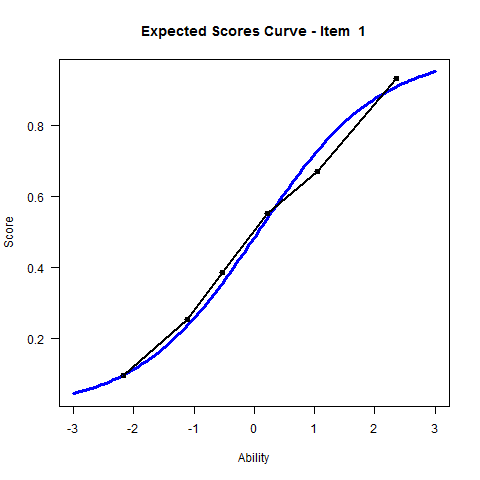
Plot Expected Scores Curves

This section shows how expected scores curves can be plotted in R. In the case of the dichotomous items, the expected scores curves are the ICC (item characterisitc curves)
           plot(mod1)

Exercises