Chapter 12 Partial Credit Models - Part II
In this session, we will learn about
- Considerations when scoring partial credit items
- Partial credit models and two-parameter models
12.1 The maximum (highest) score of an item
We frequently see that items in a test are given different maximum marks. For example, an item may be marked out of 5, while another item is marked out of 2. What are the factors that determine what maximum score an item should get? When we ask test writers about the criteria that guide them about assigning a maximum score for an item, we frequently get the following responses: “It depends on the item difficulty,” or, “It depends on how much time students need to spend answering this question.” Sometimes, the test writers look at the number of easily discernable answer categories and decide how many score points an item should be assigned.
We will say upfront that the maximum score assigned to an item should not depend on the item difficulty. This is particularly the case for multiple-choice items. When an item is difficult, there is often a lot of guessing, so that obtaining the correct answer is less likely due to high ability, but is due to some luck.
Below, we discuss about factors relating to item scores.
12.2 Item Weight, Item Information and Item Discrimination
Suppose Item 1 is scored out of a maximum of 5, while Item 2 is scored out of a maximum of 1, then Item 1 has five times the weight of Item 2 in the overall test score. That is, if you obtain the correct answer for Item 1, you get 5 points, while getting Item 2 correctly only adds 1 score point to your test score. From the test taker’s point of view, Item 1 is more “important” than Item 2, as there is an opportunity of scoring five points. From the test writer’s point of view, Item 1 should also be “important” to distinguish ability levels among students, since a higher test score should reflect a high ability. This notion of “importance” can be translated into “item information.” When an item has more “item information,” it means that it provides more power in separating low and high ability students. That is, an item with more information is a more discriminating item, since discrimination is a measure of the extent of separation of ability levels.
Consequently, we can turn the discussion around and say that items that are more discriminating should have higher maximum scores, or higher item weights in the test.
Conceptually, item discrimination and item difficulty are unrelated. That is, maximum item score should not be dependent on item difficulty, but it should be dependent on item discrimination.
A highly discriminating item is also an “important” item since it relates more closely to the construct being measured. So, in considering maximum score for an item, we can think of the “importance” of the item in terms of the construct. As an example, when we measure the propensity for developing a disease such as skin cancer, we may ask questions about skin colour, hair colour, eye colour and family history, etc. The factors that relate highly to skin cancer should get higher scores, while factors that are moderately related to skin cancer should get lower scores. We do not look at the number of categories we can separate hair colour to determine the number of score points. Instead, we need to think of how well hair colour predicts skin cancer.
12.3 Codes and Scores
In discussing response categories and scoring, we need to mention about the differences between “codes” and “scores.” We use the term “codes” to denote labelling of different response categories. While “codes” may look like 0, 1, 2, 3 etc., these codes may or may not necessarily be the scores for each response category. In fact, it will be best to have a separate set of “scores” matching the set of “codes.” For “example, we may use 0, 1, 2, 3 to code eye colour for”black”, “brown,” “green” and “blue.” But the scores for these four codes might be “0,” “0,” “1,” “2,” or, “0,” “1,” “1,” “2,” or other combinations, depending on how likely each eye colour is related to skin cancer. Nevertheless, when we are collecting data, we can use many response category “codes” to capture the data, and decide on the scores based on what the data tell us. That is, we may not assign scores to response categories a priori, unless we have information from previous studies.
12.4 PCM and Two-parameter Model (2PL)
In fact, the two-parameter model does that precisely, by estimating the weight of each item. Some two-parameter models will estimate item weights at the item level, some will estimate item weights at the response category level. For 2PL, there is a clear separation between “codes” and “scores.” In contrast, the partial credit model assigns scores a priori, and the scores are not estimated. A further difference between 2PL models and PCM is that the scores for PCM are integers, while the scores for 2PL item categories can be any real number.
12.5 An example of PCM and 2PL
In the PISA 2018 data set, one item in the student background questionnaire (code:ST197) asked students how well informed they are about a number of global issues. In particular, students were asked about
(1) Climate change and global warming (ST197Q01HA)
(2) Global health (e.g., epidemics) (ST197Q02HA)
(3) Migration (Movement of people) (ST197Q04HA)
(4) International conflicts (ST197Q07HA)
(5) Hunger or malnutrition in different parts of the world (ST197Q08HA)
(6) Cause of poverty (ST197Q09HA)
(7) Equality between men and women in different parts of the world (ST197Q12HA)
For each question, students could choose one of four options:
(1) I have never heard of this
(2) I have heard of this but I would not be able to explain what it really is about
(3) I know something about this and could explain the general issue
(4) I am familiar with this and would be able to explain this well
We have randomly selected around 5000 students’ responses to this set of questions. No student sampling weights are extracted since we will use this data set as an example for analysing partial credit items, and not for estimating proficiency levels. The data file can be downloaded here. The four options are coded as 0, 1, 2, 3. There are no missing values in this data set. The following R code analyses this data set using the PCM model. The latent construct for these seven questions is the level of students’ awareness of global issues.
rm(list=ls())
library(TAM)
library(WrightMap)
library(knitr)
gble <- read.csv("C:\\G_MWU\\ARC\\Philippines\\files\\globalawareness.csv")
mod1 <- tam.jml(gble)
thres <- tam.threshold(mod1)
Item threshold parameters (thres) are:
| Cat1 | Cat2 | Cat3 | |
|---|---|---|---|
| ST197Q01HA | -3.460602 | -1.6015320 | 1.2336731 |
| ST197Q02HA | -3.723358 | -1.0364685 | 2.0592957 |
| ST197Q04HA | -3.887970 | -1.6253357 | 1.3512268 |
| ST197Q07HA | -3.582367 | -0.9559021 | 1.7822571 |
| ST197Q08HA | -3.860138 | -1.6176453 | 1.3587341 |
| ST197Q09HA | -4.121246 | -1.7271423 | 1.0903015 |
| ST197Q12HA | -3.755035 | -1.8368225 | 0.6665955 |
The Wright Map is shown below:
w <- wrightMap(mod1$WLE, thres, item.side = itemClassic)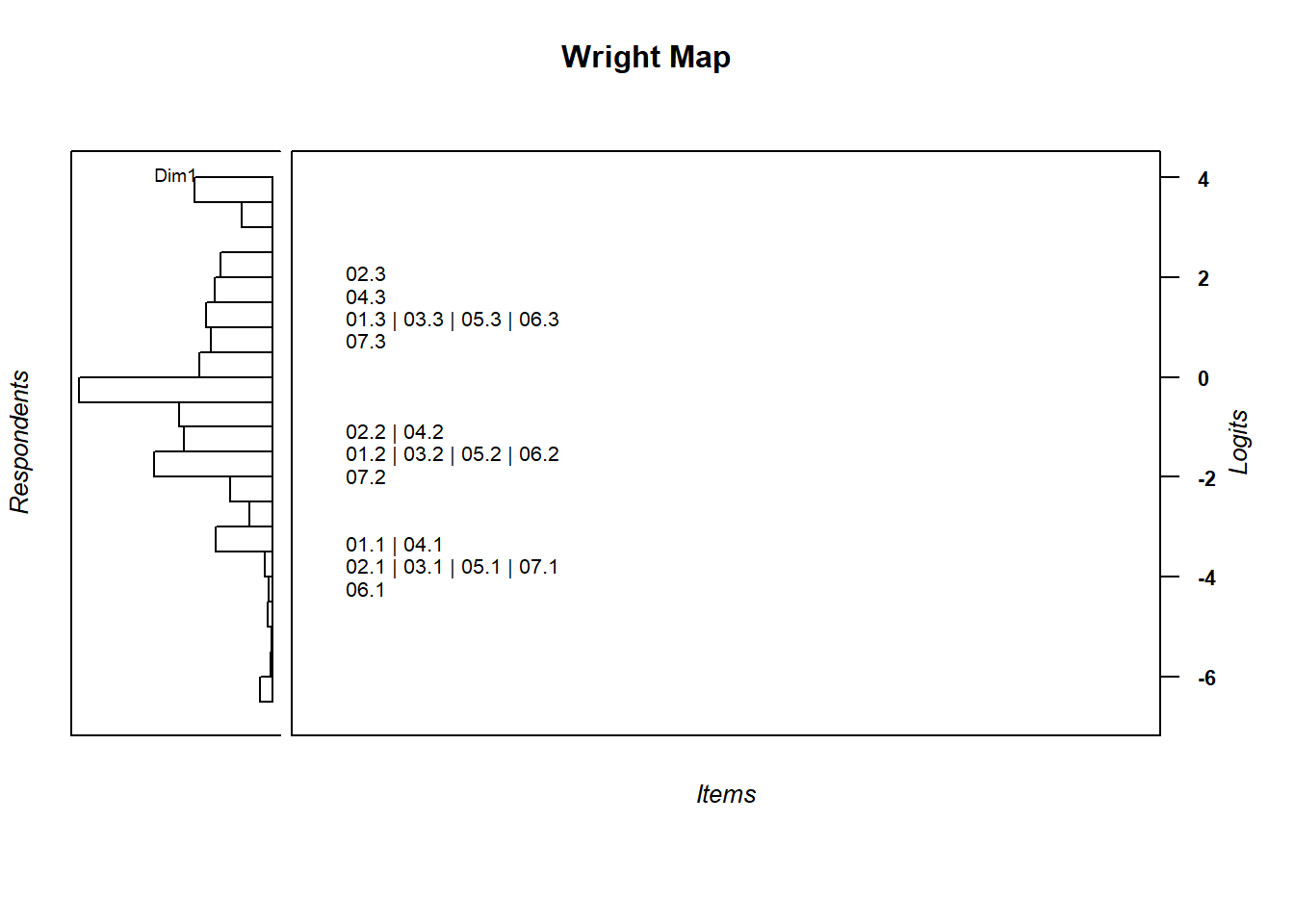
Figure 12.1: Wright Map
The ordering of the item thresholds is remarkable. The score of 1 for all items are bunched together, so are the score of 2 for all items, and score of 3. What this shows is that the item difficulty levels for all seven items are quite similar. Does this mean that we have got the scoring right? Before answering this question, let’s compute item discrimination for each item.
score <- apply(gble,1,sum)
disc <- apply(gble,2,function(x){cor(x,score-x)})
disc
ST197Q01HA ST197Q02HA ST197Q04HA ST197Q07HA ST197Q08HA ST197Q09HA ST197Q12HA
0.6178032 0.6491644 0.7038320 0.6351406 0.7207811 0.6963074 0.6324818 The item discrimination is high for all items, although some items have slightly higher discrimination. Since all items have gone through a Field Trial, it is not surprising all items are working well.
Our next step is to fit a 2PL model and estimate the “scores” for each item category. The following R code fits a 2PL model:
mod2 <- tam.mml.2pl(gble)kable(mod2$B,caption="2PL estimated item category scores/slope parameters")| Cat0.Dim01 | Cat1.Dim01 | Cat2.Dim01 | Cat3.Dim01 | |
|---|---|---|---|---|
| ST197Q01HA | 0 | 1.096437 | 2.414818 | 4.013876 |
| ST197Q02HA | 0 | 1.186946 | 2.653121 | 4.887355 |
| ST197Q04HA | 0 | 1.834553 | 3.950712 | 6.581108 |
| ST197Q07HA | 0 | 1.255264 | 2.716831 | 4.765690 |
| ST197Q08HA | 0 | 2.008038 | 4.507274 | 7.653130 |
| ST197Q09HA | 0 | 1.921985 | 4.231949 | 6.895981 |
| ST197Q12HA | 0 | 1.211725 | 2.972841 | 4.668335 |
Table 12.2 shows that the estimated item category scores for Item 5 (ST197Q08HA) could be twice that of Item 1 (ST197Q01HA). If we use the 2PL model, the item category scores are quite different across items. That is, the weightings of items are not all the same across the items, despite similar item difficulties. The test reliability in model 1 (mod1$WLEreliability) is 0.86, and the test reliability in model 2 (mod2$EAP.rel) is 0.88.
12.6 Fit statistics
The residual-based fit statistics also throw some light on the item category scoring since these fit statistics relate to item discrimination.1
mod3 <- tam.jml(gble,bias=FALSE)
f1 <- tam.fit(mod3)| ST197Q01 | ST197Q02 | ST197Q04 | ST197Q07 | ST197Q08 | ST197Q09 | ST197Q12 |
|---|---|---|---|---|---|---|
| 1.101 | 1.001 | 0.866 | 1.05 | 0.823 | 0.879 | 1.036 |
The above shows the infit mean squares for the seven items. It can be seen that the fit mean squares are lower (overfit) for items 3, 5 and 6, suggesting that these three items could have more weights. This result is consistent with the 2PL estimated slope parameters.
In summary, the item category scores in a PCM model are related to item discrimination. They are not related to item difficulty.
12.7 Homework
In the PISA 2018 released data set, one set of variables relate to home possessions. We have extract data for Questions ST012Q01TA to ST012Q09NA, and recoded the responses from “1 to 4” to “0 to 3.” Click here for the questions, and click this link for the data set. Analyse the data using the PCM model and the 2PL model. Plot Wright Map. Compute fit statistics. Make comments about which items are more difficult, and which items are least discriminating. Compare test reliabilities using PCM and using 2PL models. Make some comments about the item category scoring when using the PCM model.
Note that in the R code for calculating fit, the IRT scaling function (tam.jml) has an option of bias=FALSE. The bias correction to the item parameters is applied by default. But this bias correction will result in lower fit mean square values so they tend to be all below one, rather than centered around 1. We turn the bias correction off for computing fit here.↩︎